To use demo version of LaboTex for Windows, you must have the
following:
IBM-compatible PC.
Windows 2000/XP/2003 (Demo version also: Windows 98/Me)
Demo version is very old version of LaboTex - version 2.1 (Release 2.1.012 from April 15th, 2003).
Demo version doesn't include many new options from version 3.0 and from version 2.1.013 to 2.1.016 : ODF modelling, determination of volume fraction of texture components by model functions, skeleton lines, misorientation diagrams, ODFs comparison, ODF transformations, ODFs logical functions, pole figure grids etc. (see: 'LaboTex 2.1.015 News', 'LaboTex 2.1.016 News', 'LaboTex 3.0 News') !
The installation of demo version
To install LaboTex demo version (Labdemo2.exe -
self-extracting file), follow these directions:
Exit any applications you are running.
Select 'Run' from the 'Start' menu, find the drive
and path with the demo file, then enter Labdemo2.exe, and click 'OK'.
Read the Welcome screen, then click 'Next'. The
Software License Agreement will be displayed.
Read the Software License Agreement and again click
'Next'.
Specify a directory to install LaboTex (use short
name e.g. LaboTexd in the main directory), then click 'Next'.
Verify that the settings are correct, then click
'Next' (or use the 'Back' button if you need to go back and make
changes).
LaboTex should be installed in the destination
directory, and you will be prompted whether or not to view the README
file. Click 'Yes'.
Examples for demo tests
Demo version contains 15 examples:
Single orientation data (extension SOR):
s_orient.sor
Pole figure data (extension EPF) - with correction
file Cor(5x5).cor
C1_Triclinic.epf for C1 triclinic
crystal symmetry and triclinic sample symmetry
C2_Monoclinic.epf for C2 monoclinic
crystal symmetry and triclinic sample symmetry
D2_Monoclinic.epf for D2 monoclinic
crystal symmetry and triclinic sample symmetry
C3_Trigonal.epf for C3 trigonal
crystal symmetry and triclinic sample symmetry
D3_Trigonal.epf for D3 trigonal
crystal symmetry and triclinic sample symmetry
C4_Tetragonal.epf for C4 tetragonal
crystal symmetry and triclinic sample symmetry
D4_Tetragonal.epf for D4 tetragonal
crystal symmetry and triclinic sample symmetry
C6_Hexagonal.epf for C6 hexagonal
crystal symmetry and triclinic sample symmetry
D6_Hexagonal.epf for D6 hexagonal
crystal symmetry and triclinic sample symmetry
T_Cubic.epf for T cubic crystal symmetry and
triclinic sample symmetry
O_Cubic.epf for O cubic crystal symmetry and
triclinic sample symmetry
O_Cubic_C2.epf for O cubic crystal symmetry and
monoclinic sample symmetry
O_Cubic_D2.epf for O cubic crystal symmetry and
orthorhombic sample symmetry
O_Cubic_Arb.epf for O cubic crystal symmetry and
arbitrary beta range
To select example:
Choose 'New Sample' from the menu 'File' or the
toolbar,
Choose an appriopriate experimental data file (EPF or
SOR)
Select the correction file (COR(5x5).COR) (only for
EPF files)
Change sample name (because demo contains calculated
CPF file with the same name)
Choose 'Create' button and 'Run' button (in the next
dialog) to build:
CPF objects 'HKL' (CPF - experimental pole
figures data after correction + initial normalization). As a result
you create only CPF objects for the chosen sample (CPF icon will be
activated - neighbour icons on the second toolbar are grayed). CPF
objects are the basic data for the ODF calculation from pole
figures.
or
ODF object (in case of the single orientation
data SOR). In this case ODF icon will be activated - neighbour icons
on the second toolbar are grayed)
The ODF calculation
If a sample contains CPF objects (CPF icon is activated - all
samples in the demo version contain calculated CPF objects), you are able to
calculate ODF. To do that choose 'CPF to ODF,...' (using menu 'Calculation'
or icon on the toolbar). Before begining the ODF calculation you may (using
the dialog window from the right side):
change optional parameters which will finish
calculations (number of iteration steps, minimal RP and dRP errors),
add or remove pole figures from the ODF calculations
by pressing 'hkl' buttons (ODF is calculated only from visible pole
figure(s)),
perform appriopriate symmetrizations of pole figures,
change upper and lower range of the pole figures
selected to ODF= calculation,
rotate pole figure(s).
To begin the ODF calculation press the button 'Run ODF
Calculations'. The following objects are built at the end of ODF
calculation:
NPF (normalized experimental pole figures - these
figures differ from CPF by normalization factors, NPF are normalized on
the base of the ODF),
RPF (pole figures recalculated from ODF with 'HKL'
corresponding to that one selected for ODF calculation),
INV (inverse pole figures (XYZ) : (100), (010),
(001)).
You can see that sample contains new objects which are
symbolized by activated icons on the second toolbar: ODF, NPF, RPF and INV.
You can calculate next ODF for the set of new parameters. In this case a new
job will be created (on the second toolbar will be displayed new buttons
'J1', 'J2' ...). For one sample you can have maximal 9 jobs.
The ODF symmetrization
You can do a symmetrization of calculated Orientation
Distribution Function (ODF) to a monoclinic, orthorhombic or axial sample
symmetry. This option can be selected from the 'Calculation' menu or by
pressing the appropriate icon on the toolbar.
APF and INV calculation
You are able to calculate additonal pole figures (i.e. pole
figures, which were absent in the ODF calculation) and inversion pole
figures when the sample contains calculated ODF (in that case ODF icon is
activated). Choose 'ODF to APF' or 'ODF to INV' (using the 'Calculation'
menu or icon on the toolbar) to open dialog for APF and INV calculations.
Display of different type of the LaboTex objects -
Compare Mode
Labotex operates on six types of the LaboTex objects:
CPF - Corrected Pole Figures
NPF - Normalized Pole Figures
RPF - Recalculated Pole Figures
APF - Additional Pole Figures
INV - INVerse pole figures
ODF - Orientation Distribution Function
These six types of objects can be stored in three types of
containers:
The Pole Figures Container for CPF, NPF, RPF, APF
objects (yellow colour icon)
The Inverse Pole Figures Container for INV objects
(blue colour icon);
The Orientation Distribution Function container for
ODF objects (green colour icon).
The toolbar with objects is displayed on the top of the
application window, below the Main Toolbar. The toolbar provides quick mouse
access to the LaboTex object (selecting: hkl - for pole figures, XYZ - for
inverse pole figures and type of projection for ODF). Number of objects in
the containers are indicated in the left bottom corner of the window (
yellow colour number for pole figures container, blue colour number for
inversion pole figures and green color number for orientation distribution
function container). Only one projection can be in the container of the ODF
objects simultaneously. For the ODF container, the number indicates the
number of 2D ODF sections. Pole figures type objects (CPF, NPF, RPF, APF),
inversion pole figure type objects (INV) and orientation distribution
function (ODF) type objects can not be displayed in one window
simultaneously. You can display different type objects using 'Compare Mode'
(using 'View' menu or icon on the toolbar). In the compare mode you can work
in two windows using different or the same type of objects. In this mode
following options are not active:
calculation (ODF, APF, INV);
creation of new sample (CPF);
quantitative analysis.
Orientation analysis
You can do orientation analysis for pole figure objects (CPF,
NPF, RPF, APF) and ODF objects. You can not do analysis for inversion pole
figures objects. For different type of objects (PF and ODF) you have to use
'Compare mode' (using 'View' menu or icon on the toolbar). The Compare mode
is very important for education (interdependence of orientations on PF and
ODF).
Choose 'Orientations Analysis' from menu 'Analysis' to begin analysis. Cross
marks indicate positions of orientation. On the second toolbar you can see
orientation in HKL UVW and Euler angles. Using buttons from the second
toolbar, you can move cross mark(s).
You may write angles or indices of orientation directly into the text
windows on the toolbar.
On the ODF projection you may click on the diagram that moves a cross mark
and shows appriopriate orientation.
To see the value of intensity for the selected orientation (indicated by
cross marks on ODF or PF diagram) you can select 'Show PF or/and ODF Value'
(using 'Analysis' menu or 'V' icon on the toolbar) . Value of ODF or/and PF
(see help) are displayed on the status bar (sums PF value(s) or/and ODF
value in cross mark(s) position(s), for more than one of PF objects -
average of sums).
Attention ! In orientations analysis mode '3D View' is not active.
Qualitative Analysis
To do qualitative analysis, choose appriopriate objects and
next press 'SORT' button on the bottom toolbar or 'Sort of Orientations from
Database' using 'Analysis' menu. You will see the window with assorted
orientations from database by PF or ODF values (+ one additional orientation
for current cursor position).
You can also analyse near (HKL)[UVW] orientations. Select "Orientation
analysis". Click right mouse button in selected point on the pole figure or
ODF projection. This option can be chosen from analysis menu too. "Near
orientations" can be sorted by PF or ODF values, Miller indices or distance,
Quantiative analysis
Quantitative analysis is possible only in a single mode for
selected ODF projections.
Quantitative analysis makes possible to calculate volume fractions of chosen
set of texture components.In order to complete the quantitative texture
analysis, the following steps are recommended:
display one of ODF projections,
identify the texture components (showing orientations
from database and/or identifying orientations components by manual
movement of the cross mark),
select 'Quantitative Analysis' from 'Analysis' menu
or press '%' icon on the toolbar
select texture components (orientations) for
integration of volume fractions
select the integration width (change slider position)
of each Euler angle for selected components
press 'Calculation of volume fraction of texture
components' button
Orientations type database
You can add orientations to the database selecting
'Orientations Type Database' from the 'Analysis' menu .
It allows to edit or delete orientations from database.
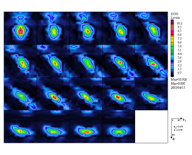
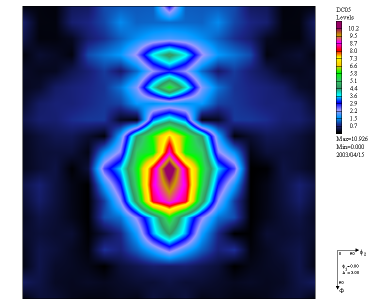
Calculated example
The sample O_Cubic.epf contains the following calculated
objects:
CPF (experimenatal corrected pole figures);
ODF (orientation distribution function);
NPF (normalized experimental pole figures);
RPF (recalculated pole figures from ODF);
INV (inverse pole figures).
If you choose O_Cubic sample using 'Open sample' from the
'File' menu or icon on the toolbar then on the second toolbar there should
be activated icons of CPF, ODF, NPF, RPF and INV objects. Select one of them
and display the appropriate object by pressing one of the activated buttons
respectively.
For other examples containing pole figure data (CPF), you may calculate the
ODF (and NPF, RPF, INV simultaneously). CPF objects can be recalculated
(with changed sample name if you wish) from experimental data (EPF object).
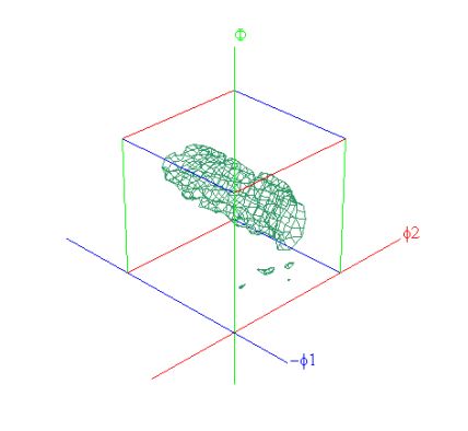
3D View
You can view objects in 3 dimensions choosing '3D View' from
'View' menu or '3D' icon on the toolbar.
This option is available for main window only.
Objects description
Clic the right mouse button to view of objects descriptions.
Selected object
Click the left mouse button to select an object. Selected
object is in red a frame and appriopriate button contains red text. If
current sample is different than selected object sample, the LaboTex changes
current sample. You can delete or magnify selected objects. Mmagnify an
object by clicking twice on it (in ODF you can magnify one section of the
projection).
Show of basic region of PF
Basic region means:
half circle of PF in case of monoclinic sample
symmetry,
quarter circle of PF in case of orthorhombic sample
symmetry
2D radial section of PF in case of axial sample
symmetry.
New manuals are available (please download from www.labotex.com):
"Fundamentals of 3-D Texture Analysis ";
"Hexagonal Axes: Conventions & Conversions"
"LaboTex: Skeleton Lines and Misorientation Diagrams"
New data formats (details you can find in www.labotex.con --> 'Data Formats'):
with extension 'HPF' - experimental data: pole figures;
with extension 'CSV' - Oxford Crystal Single Orientations File 3);
with extension 'ASC' - Seifert PTS 3000 ASCII data format - experimental data: pole figures;
with extension 'TXT' - Rigaku 3014 - ASCII data format - experimental data: pole figures;
'XML' - format - files should to have extension 'XRDML' - PANalytical XML data format.
'EXP' (RWTH Achen).
Analysis of Inverse Pole Figures: LaboTex shows {hkl} in place of the cursor position on the complete inverse pole figure
and on the partial inverse pole figures. LaboTex shows Miller-Bravais indices {hkil} for hexagonal and trigonal crystal systems.
Simultanously LaboTex shows Inverse Pole Figure Intensity in cursor position and position in alpha and beta angles.
New Dialog 'Max. Value of Miller Indice' in menu 'Analysis' allows to set maximal value of Miller or Miller-Bravais indice in the range '5' to '15'.
This dialog is important during analysis of Inverse Pole Figures when you want to find only {hkl} or {hkil} with indices
lower than default (i.e. '15').
LaboTex calculates 'f' texture factors defined by JJ Kearns ( JJ Kearns 'Thermal expansion and preferred orientation in Zircaloy',
Bettis Atomic Power Laboratory, Report WAPD-TM-473,1965 and JJ Kearns, CR Woods, J. Bucl. Mater. 20 (1966) 241).
The 'f' factors have found use for correlations and materials characterization of hexagonal materials
(thermal expansion, irradiation growth,elastic properties in zirconium and titanium alloys).
LaboTex calculates these factors also for Orthorhombic and Tetragonal Crystal Systems.
'f' factors inform us about fractions of basal pole [0001] (or [001]) in each if three principal directions :
X (RD), Y (TD) and Z (ND). Perfect alignment of the basal poles in one direction gives an 'f' value of
'1' in that direction and '0' in second and third directions. The sum of 'f' factors in the three directions is equal 1.0.
You can start Calculation of 'f' Factors from menu 'Calculation'.
Fixed problems in hexagonal system for second convention (model calculation, transform ODF calculation) and for inverse pole figure plot when first convention were used.
New dialog for data format with extension 'TXT' for input of single orientation data files. Now user can choose
Nos of columns for: Phi1, Phi and Phi2 angles. User can also choose unit of angles: degrees or radians.
User can save data for sections, skeleton lines and misorientation diagrams.
Corrected ODF transformation from rotation model for crystal symmetry lower than cubic (ODF transformation was incorrect for some 'hkl' vectors).
Texture index is displayed with resolution 3 digits after point. It is important for determination of quality of texture 'free' samples (samples for defocussing correction).
Corrected displaying of volume fraction in MFM for small values of volume fraction (<0.5%).
UXD data format allows many pole figures in files (for details please see to ->Data Formats).
Corrected description of ODF transformation in ODF report.
Fixed problem with ODF export (lack of data for maximal Phi1 angle).
Fixed also several other small problems with presentation of pole figures and others.
News in version 3.0.02.
In version 3.0 of LaboTex you can find many tools for comparison of ODFs (up to 12 ODFs) and for comparison of pole
figures (also up to 12 pole figures).
ODF line sections (cuts) - user define two points in Euler Space (Screen Shot).
LaboTex shows ODF intensity along section defined on the base these points.
User can also choose initial points from orientations database (when click on the 'Start Point' or 'End Point' button database is available (Screen Shot) ).
Comparison up to 12 ODFs is possible, (Screen Shot)
skeleton lines (Screen Shot). - user can create such diagrams as: alpha-fiber, beta-fiber, gamma fiber etc..
User can choose skeleton lines on the base of Euler angle (Phi1, Phi or Phi2) and:
misorientation histograms.(Screen Shot)
User define start point in Euler Space from which LaboTex shows misorientation diagrams.
Misorientations diagrams are calculated on the base of ODFs in range 0 to 80 deg from start point (start orientation).
LaboTex shows intensity which is the releative intensity i.e.intensity relate to intensity of random sample (I=I(sample)/I(random sample))
for the same range of misorientation angle. User can make comparison up to 12 misorientations histograms.
User can also change histogram step in range 1 to 10 degrees;(Screen Shot)
There are many options to optimalize quality of diagrams :
scale (in percent of maximal intensity value: 0.1 up 100%) (Screen Shot);
colors (defined by user);
types of lines (14 types with different dots+solid) (Screen Shot);
line options (all solid, all black, black countours) (Screen Shot);
User can also save current parameters and/or samples (Screen Shot).
The first ODF is current ODF. Next ODFs for comparison user can choose using
appriopriate comboboxes and buttons on the tools window from right side. (Screen Shot);
ODFs - logical operations. (Screen Shot)
For activate this option user should switch LaboTex to Compare Mode and next choose two ODFs for comparison: one in left window and second in
right window (LaboTex Compare Mode).
On the base these two ODFs (A - from left window and B from right window) LaboTex creates new ODF which is:
intersection of ODF A and ODF B,
diference of ODF A and ODF B (or B-A),
union of ODF A and ODF B,
sum of ODF A and ODF B,
ODF difference : A or B - intersection A and B,
inverted ODF (only for A).
New ODF is created in new Job for sample of ODF A.
You can copy and paste these diagrams to other applications or you can made images in 'BMP' ot 'TIF' format (menu 'Edit').
Transformations of ODF. LaboTex calculates new ODF which is results transformation of initial ODF. New ODF is created in new job for sample of initial
ODF. There are two kinds transformations:
builder of model rotations, (Screen Shot). (crystalites/planes rotations). In first step you build rotation model and save it.
In rotation model you can choose up to 10 orientations for which you set:
ranges of Euler angle around center of orientation (and for symmetrically equivalent positions);
vector "hkl" around which will be rotate crystalites/planes (only these which are included in ranges chosen by user);
rotation angle;
recent of rotated crystalites/planes (from 0 to 100%).
In second step you choose rotation model and make ODF transformation (Screen Shot).
Generation of single orientations (Screen Shot)
: LaboTex creates set of single orientations on the base of current ODF.
User can choose number of single orientations from 10000 to 9999999. This option is important for user which modelling deformation (VCS users) etc.;
User can also generate random set of single orientation using this option. SOR file creates by LaboTex user can input as a new sample and
he can make ODF calculation. Examples:
ODF creates on the base set of 500,000 single orientations generates with 'Random' option.
(Screen Shot).
Section of pole figure {111} calculated on the base above 'Random' ODF. (Screen Shot).
Comparison pole figure for real texure free (random) sample (red) with pole figure generates from 'random' ODF creates on the base set of 500,000 single orientations (blue)
(Screen Shot).
Pole figures sections (cuts). User defines start and end points on the pole figure
and Labotex shows intensity along this section (Screen Shot).
There are following cuts available:
'Radial (full)' (in range 90 - 0 - 90 degrees) (Screen Shot).
LaboTex shows position of section line on the pole figure when button 'View' is pressed (Screen Shot).
Up to 12 pole figures can be comparised. All information about comparised PFs are displayed in infor window from left side (Screen Shot).
All pole figures which section are displayed have to be choosen before button '2D' has been pressed.
(if you choose more than 12 pole figures then LaboTex shows only first 12 pole figures sections).
There are many options to optimalize quality of diagrams :
scale (in percent of maximal intensity value: 0.1 up 100%) (Screen Shot);
colors (defined by user);
types of lines (14 types with different dots+solid) (Screen Shot);
line options (all solid, all black, black countours) (Screen Shot);
You can also save current parameters (Screen Shot).
You can copy and paste these diagrams to other applications or you can made images in 'BMP' ot 'TIF' format (menu 'Edit').
On-line view of alpha (radial angle), beta (azimuthal angle) and pole figure value in mouse cursor position.
LaboTex display this data in format: (alpha,beta) PF='value of PF'. Only in case, when mode of LaboTex is switched to 'Cursor Analysis'
and toolbar button 'Show Value(s)' is pressed LaboTex shows of sums PF value(s) in pole positions which are indicates by cursors
(mark by small crosses) (for more than one of PF objects - average of sums).
; (Screen Shot)
New column in "Near {HKL}< UVW>" window has been added: column with misorientation angles
(misorientation beetwen {HKL}< UVW> and cursor position on the ODF diagram).
(Screen Shot).
Intel® has solved problem with combability their
graphic driver with LaboTex. If you are using Intel® graphic (Intel®
830M/MG,845G/GE/GL/GV,Intel® 852/855, GM/GME,865G) then please download
new driver (Version 14) from Intel® WWW pages:
Download New Intel® Graphic Driver (Version 14)
LaboTex Version 2.1.016 news (11.2003)
Option "Once" in volume fraction calculation is
active now (calculation of relative error between model ODF and
experimental ODF).
New option has been added as default: "Max.
linearity" in calculations of a model ODF. LaboTex chooses orientation
(among sym. eq. orient. of component) for model building which lies in
maximal linear area of ODF. This option is essential only for cubic
crystal symmetry.
Corrected bug in volume fraction calculation
(integration method) - volume fraction for components with sym. eq.
orientations lying on phi=0 (for example: Cube) was elevated when there
were also other components with sym. eq. orientations lying close
phi=90.
Option "User defined .." in menu Edit for skeleton
lines plots is grayed now.
LaboTex Version 2.1.015E news (10.2003)
Model function method determination of volume
fraction of texture components (texture approximation by model
components). Screen Shot - Model Function
Method - Dialog Window
Now, you can in LaboTex make calculations of volume fraction of texture
components using two independent methods:
Visualization of background and manual setting of
background (fon) in volume fraction calculation (Integration Method). In
previous versions of LaboTex, LaboTex set up value of background to
minimal value of ODF in integration method of volume fraction
calculation. Now, minimal value of ODF is set up for default only and
user can change this value. Screen Shot - visualization of
background and manual setting of background
New options for input data: When background data of
pole figure is greater than pole figure data for some values LaboTex
makes:
a) negative values of pole figure after correction for background are
set to zero.
b) adds to all pole figure data absolute value of the lowest values of
pole figure after correction for background (LaboTex makes all data
positive); User may choose option a) or b) in "LaboTex Option" ---->
"Data Formats". Default is option a). Screen Shot - The choice of
option for background of pole figure
Now, LaboTex informs user's when it finds data for which background data
are greater than pole figure data and LaboTex display percent these data
(Example).
New format - "DAT" to input data from Seifert XRD
(one pole figure for one file).
New format - "COA" to input data (one pole figure for
one file).
New version of "UXD" format (compatible with
multexarea).
The possibility of setting maximal value of Miller
indices in conversion from Euler angles (in the range 5 to 15).
(Example)
Improve precision of integration in determination of
volume fraction of texture components (Integration Method).
Corrected documentation: "The Nomenclature of Inverse
Pole Figure Use in LaboTex".
Changes in conversion of data format from PHILIPS
XRD: "TXT" and binary "RW1".
LaboTex input data for different azimuthal and radial
steps (azimuthal step is adjusted to radial step by linear
interpolation). Azimuthal step has to be in the range 1-10 deg., radial
steps as in previous versions (see to: 'LaboTex Specification').
Warning: Option "User defined .." in menu Edit and
option "Once" in volume fraction calculation are inactive.
LaboTex Version 2.1.012 news (15.04.2003)
Visualization of Inverse Pole Figure in the standard
stereographic triangle (partial inverse pole figure, inverse pole
figures in basic region) for :
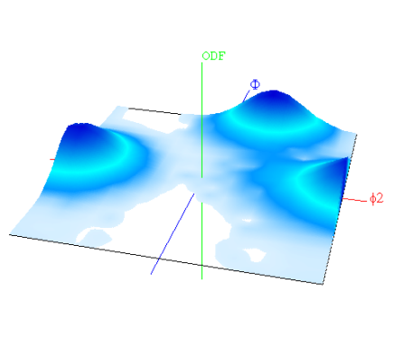
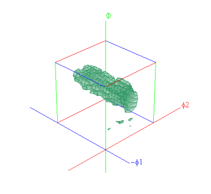
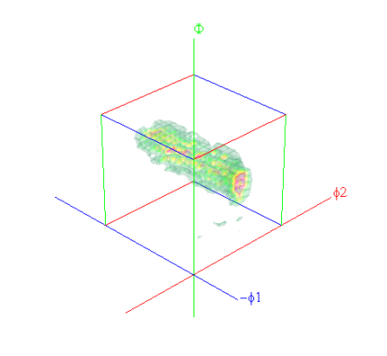
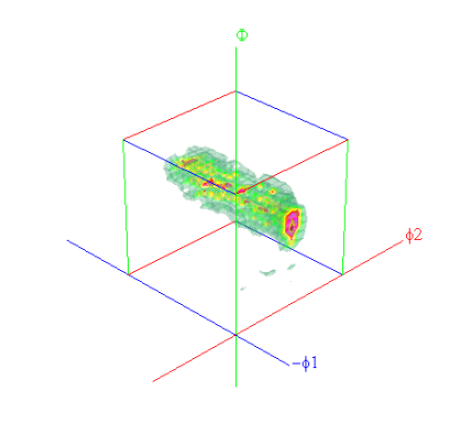
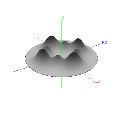
"Continuous" 2D and 3D visualization of pole figure,
inverse pole figure, ODF section and ODF (full color visualization on
the base of the value of each point of the object. In 3D visualization
height in each point is a function of PF,IPF or ODF value). Very good
option in presentation and in publication. WARNING: This option needs
installation of OpenGL Driver for your graphic card! Printing plots in
this option may be longer. Choose: 'Fill' next 'Open InfoBox' and in
fill option change from 'Normal' to 'Continuous' in Isoline Combo Box.
Example:
WARNING: LaboTex has and ever had user defined
legend. Default is "Automatic". User may change to "Manual" or to any
user defined files with isoline values. For example and details see to
"Determination of Volume Fraction of Texture Components Using LaboTex"
manual. User can save in every time current isolines . It is very
important compare objects the same type for the same set of isolines.
LaboTex Version 2.1.011 news (17.01.2003)
New data format "NJA" - Seifert ASCII data format.
Each pole figure and background file has to be in separate file with
extension NJA.Pole figures data files are input from "Choose
Experimental Data" list and defocussing correction data (random pole
figures data) can be input if necessary from "Choose Defocussing
Correction" list. 'NJA' files contain background data (additional files
with background data are unnecessary).
The possibility of the evaluation of parameters of
component peak. New slider in Quantitative Analysis which allows
magnification of component peak and manually evaluation its parameters
(heights, FWHM...).
Labotex can read background files for UXD format:
data for background please mark with 'B' letter in indices of pole
figure ( in filename - for example '<111B>corund'). LaboTex
requires one pole figure on the one UXD file. Each pole figure and
background file has to be in separate file with extension UXD.For
example: sample_100.UXD, sample_100BL.UXD, sample_100BR.UXD, ... (files
with terminations BL or BR are background from 'left' and 'right' side
of PF. LaboTex average BL and BR values). You may use only BL or BR
file, too. Background files in UXD format are allowed only one
background value for one alpha value.
Fix problem with symmetrically equivalent
orientations for some fiber components. For example: for component
<511>fiber LaboTex shows only <511>fiber and <151>fiber sym. eq. Now
LaboTex shows all symmetrically equivalent orientations: <115>fiber,
<511>fiber and <151>fiber.
Extended format for display value of isoline and
maximal value of ODF. Now it is long enough even for very sharp
textures.
Fix problem in compare - high resolution mode with
display ODF values.
LaboTex Version 2.1.010 news (22.10.2002)
The user may turn on or turn off high resolution ODF
mode.Please, turn on high resolution mode to calculation of volume
fraction using high resolution ODF.
Limit of high resolution mode lowered from 3.0x3.0 to
2.5x2.5 deg. Now high resolution mode include range from 1x1 to 2.5x2.5
deg.
Fix problem with calculation ODF for symmetrization
to axial and resolution equal or lower than 3.0x3.0 (in high resolution
mode).
The choice among Roe and Bunge notation in data
format ANG, CTF, SNG, TSV, TXT.
Fix problem with UXD files.
LaboTex Version 2.1.009a news (11.10.2002
- extended version 2.1.009)
New options in calculation of volume fractions.
Calculations of volume fraction of chosen texture components are
performed by integration around those components in basic region. Each
components can be represented by more than one symmetrically equivalent
position (orientations) in basic region. Fundamentals for calculation of volume fraction of texture
components:
LaboTex makes integration around each orientation
in the ranges delta chosen by the user for each Euler angle:
Phi1-delta(Phi1) to Phi1+delta(Phi1),
Phi-delta(Phi) to Phi+delta(Phi),
Phi2-delta(Phi2) to Phi2+delta(Phi2),
In the case of exit outside the basic region of
ODF space (Euler angles space) LaboTex continues integration in
equivalent area of the basic region.
The overlapping problem
The overlapping problem appears when integration ranges (delta) are too
wide or when orientations are near each other in Euler angles space.
Integration area of texture components can be overlapped in two ways:
i) Overlapping of integration ranges between symmetrically equivalent
positions of component
ii) Overlapping of integration ranges between different components
LaboTex gives three different abilities (strategy) to solve problem of
overlapping of integration ranges between symmetrically equivalent
positions of component (case i) :
"Simple Integration" - overlapping region is
multiply integrated. Integration around any single component in full
range of basic region gives (100% minus background)*number of
symmetrically equivalent position.
"Singlely Counts in Overlapping Area" -
overlapping region is only singlely integrated for component.
Integration around any single component in full range of basic
region give 100% minus background.
"Divide by Number of Symmetrically Equivalent
Position" - LaboTex integrates for all symmetrically equivalent
positions of the components with proper weight equal 1/number of
symmetrically equivalent positions. Integration around any single
components in full range of basic region give 100% minus background.
To solve problem of overlapping of integration ranges between different
components LaboTex offers (case ii):
Total percent of overlapping (overlapping volume
fraction) is displayed in special window ("Orientations Overlap").
Overlapping volume fraction can be limited by diminishing
integration ranges of texture components.
In case of "Simple Integration" overlapping
volume fraction means sum of overlapping between different
components and between symmetrically equivalent positions of all
overlapped components.
In case of "Singlely Counts in Overlapping
Area" overlapping volume fraction means sum overlapping between
different components.
In case of "Divide by Number of Symmetrically
Equivalent Position" overlapping volume fraction means excessive
orientation overlap. Excessive orientation overlap area is
defined in the points where sum of weights is greater than 1.
The weight is equal to 1/number of symmetrically equivalent
positions. Excessive ODF value in given point is equal to the
product of the ODF value and sum of weights minus 1. The volume
fraction of excessive orientation overlap is the integral of
excessive ODF values in mentioned area.
Overlapping volume fraction can be divided among
overlapping orientations. This option causes the division of ODF
values from overlap areas among overlapping orientations:
in case of "Simple Integration" and "Singlely
Counts in Overlapping Area" ODF values in overlapping areas are
divided proportionally to number of symmetrically equivalent
overlap orientations.
in case of "Divide by Number of Symmetrically
Equivalent Position" excessive ODF values in overlapping areas
are divided among components proportionally to the weights and
to number of symmetrically equivalent overlapping orientations.
Fix problem with false information about not enough
free space on the disk.
Fix problem with UXD files.
Now LaboTex shows minimal and maximal value of
objects (PF,INV and ODF) separately for left and right window in the
Compare Mode.
Improved the refreshment of the screen after the
change of colours in the Compare Mode.
LaboTex Version 2.1.009 news (26.09.2002)
Quantitative and qualitative texture analysis for
samples with axial pole figures symmetry.
The Analysis of fiber orientations:
fiber orientations can be added to the LaboTex
database,
ODF values in qualitative analysis (SORT option)
for fiber orientations are averaged along fiber direction,
LaboTex shows fibre orientations on pole figures
or ODF after using "UVW" button on the toolbar or selecting
orientation from orientations combo box,
the volume fraction for fiber orientations can be
calculated together with ordinary orientations,
the considerable acceleration of calculation in
quantitative and in qualitative analysis,
indicating of near (HKL)[UVW] orientations. Select
"Orientation analysis". Click right mouse button in selected point on
the pole figure or ODF projection. This option can be chosen from
analysis menu too. "Near orientations" can be sorted by PF or ODF
values, Miller indices or distance,
placing of the selected pole in indicated position on
pole figure. Select "Orientation analysis". Click left mouse button in
selecting point on the pole figure.
Now LaboTex can read data in 4 new data formats:
XPF - BEARTEX data format (corrected pole
figures)
Pole figures data files: *.xpf (input from
"Choose Experimental Data")
PFG - RIST data format from RIGAKU (ASCII)
Pole figures data files: *.pfg (input from
"Choose Experimental Data" list)
Random pole figures data files: *.pfg (input
from "Choose Defocussing Correction" list)
txt - RIST data format from PHILIPS (ASCII-
corrected pole figures)
Pole figures data files: *.txt (input from
"Choose Experimental Data" list)
RW1 - PHILIPS XPert binary data format (Binary)
Pole figures data files: *.rw1 (input from
"Choose Experimental Data" list)
Background pole figures data files: *.bgr
(input from "Choose Experimental Data" list)
Defocussing correction data files: *.cor
(input from "Choose Defocussing Correction" list)
Please choose required format in LaboTex Options. If
extensions of files with data differ from higher indicated please to
change it on correct.
Now LaboTex is able to import data in 24 data formats!
Only orientations type are changed and indicated in
'AUTO' mode (during orientation analysis for pole figures).
Now LaboTex makes printable reports from
qualitative and quantitative calculations.
Now LaboTex shows diagram of ODF values around all
symmetrically equivalent orientations (in quantitative analysis). Please
click on the proper position on the list box.
Corrected calculations of ODF for axial symmetry.
Improved the usage of set of orientations in
quantitative analysis
LaboTex Version 2.1.008 news (29/03/2002)
Save PFs and ODF images as bitmap files: BMP,TIF
(width, height and resolution of image can be given by user selection),
Copy to clipboard as a bitmap in 2-D and 3-D (printer
or screen resolution!!!),
The possibility of the choice of the axis convention
in hexagonal system,
Numerical settings in 3-D (distance, rotation, shift,
axis lengthening (abbreviation)),
LaboTex allows negative indices in additional pole
figures calculations,
Now, arrangement of objects on the printer output is
the same as on the screen,
Small changes of the appearance toolbars.
LaboTex Version 2.1.007 news
LaboTex allows negative indices for pole figures
LaboTex Version 2.1.006 news
LaboTex convention for sample and crystal coordinate
system - from version 2.1.006 (change important in Euler to Miller
conversion and Miller to Euler conversion for symmetry lower than cubic
symmetry):
1) X,Y,Z axis perpendicular to each other,
2) [100] axis is in XZ plane,
3) Z axis is paralel to the [001]
crystallographic plane,
4) Crystal coordinate system and sample
coordinate system should be at the same order i.e. both right-handed
or both left-handed,
5) Bunge definition of Euler angles.
Now, LaboTex shows exactly and approximately
orthogonal vectors {HKL}< UVW> for indices lower than 15 (eliminates
"Non orthogonal" information). Conversion Euler angles to Miller indices
is made on the basis of cell parameters of sample (in compare mode - on
the basis of cell parameters sample from active window). If pole figures
in active window have different cell parameters conversion is made on
the basis of cell parameters of sample which pole figure is first in
active window.
Now basic area for pole figures is equal to a full
range of Euler angles hence number of orientations in basic area (in
combo box) can be different for ODF and PF objects.
The window for set up {HKL}< UVW>.indices has been
changed. Now you can see for active window: cell parameters, orientation
type (Euler angles and Miller indices), basic region, orientation(s) in
basic region (Euler angles and Miller indices).
New samples for hexagonal symmetry
Fix error in "Copy to clipboard" in low resolution
Fix error in save isolines (for isolines > than
odf-max or pf-max)
Fix error for long LaboTex path
Fix error : inactive compare mode when user changes
symmetry after opening LaboTex